(Blog-translation)What are Diffusion Models?

lilianweng.github.io - What are Diffusion Models?

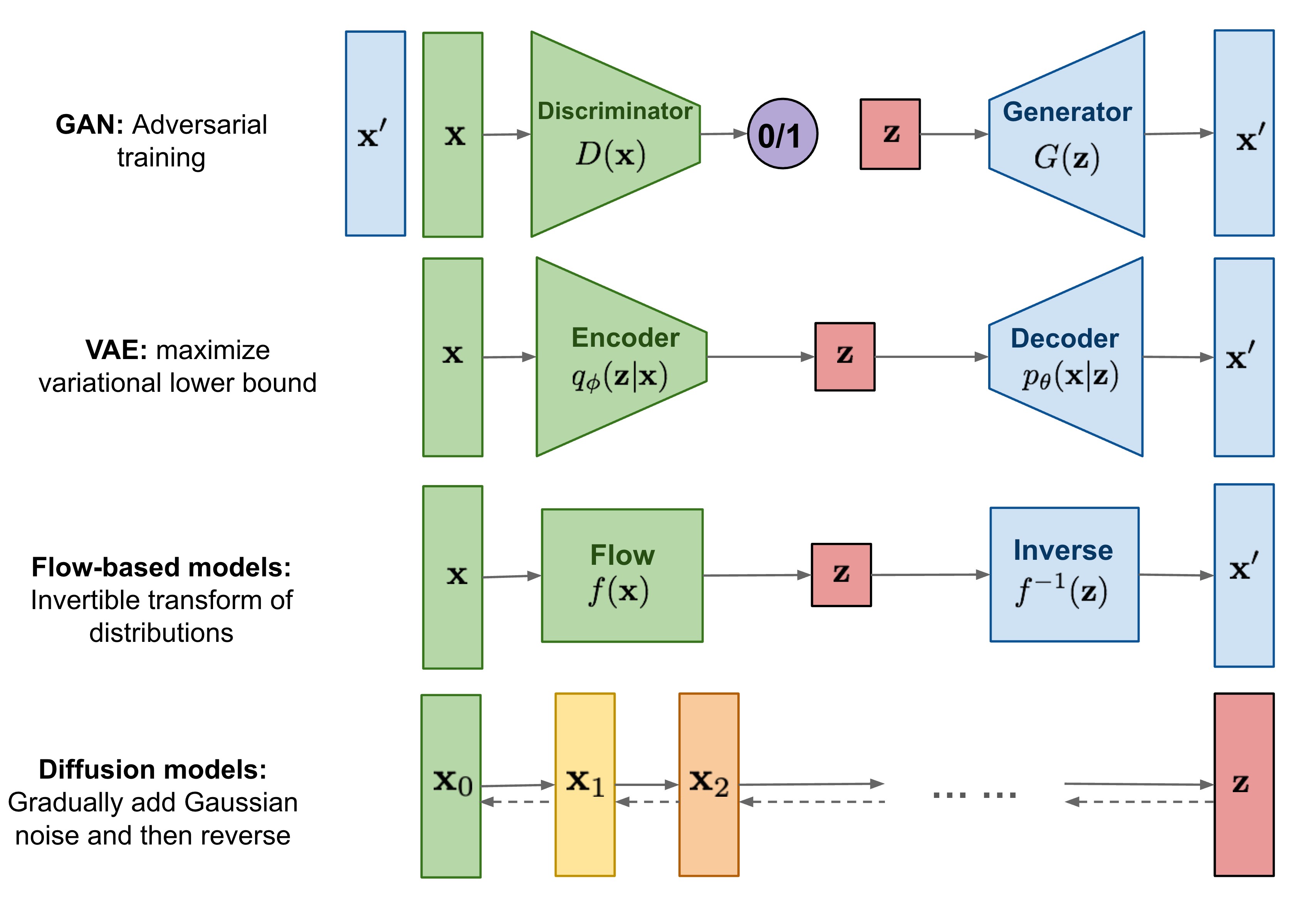
So far, I’ve written about three types of generative models, GAN, VAE, and Flow-based models. They have shown great success in generating high-quality samples, but each has some limitations of its own. GAN models are known for potentially unstable training and less diversity in generation due to their adversarial training nature. VAE relies on a surrogate loss. Flow models have to use specialized architectures to construct reversible transform.

지금까지, 나는 세가지 generative model(생성 모델)들인, GAN, VAE 그리고 Flow-based 모델들을 포스팅 했다. 그것들은 성공적 high-quality 결과들을 잘 생성함을 보여준다. 하지만 모델들 각각에는 한계가 존재한다. GAN은 adversarial 훈련의 성격상 결과를 생성할 때 근본적으로 불안전한 훈련과 적은 다양성으로 알려져있다. VAE는 surrogate loss^[1]에 의존한다. Flow-based model은 가역적 변환(reversible transform)^[2]을 구성하기위해 특별한 아키텍쳐를 사용해야한다.

1. VAE의 surrogate loss란?
   • VAE의 surrogate loss란, VAE에서 학습을 위해 사용되는 대체 손실 함수를 말합니다. VAE에서는 생성 과정에서 발생하는 손실 함수를 직접 최적화할 수 없기 때문에, 대신 최적화 가능한 다른 손실 함수를 사용합니다. 이러한 대체 손실 함수를 surrogate loss function이라고 합니다. [1-1]
2. Reversible transform
   • Flow-based 모델에서 Reversible transform은 역변환 가능한 invertible function(가역함수)^[3]로, 입력과 출력을 모두 재생성할 수 있습니다. 이러한 역변환 가능한 특성을 이용하여 데이터 분포를 학습하고 생성하는데 활용됩니다. 이는 Generative model에서도 많이 활용되는데, 이를 통해 실제같은 이미지 생성이 가능해집니다. Reversible transform은 1x1 Convolution, NICE(Non-linear Independent Components Estimation), RealNVP(Real-valued Non-Volume Preserving) 등 다양한 방식으로 구현될 수 있습니다.[2-1][2-2] Flow-based 모델에서 Reversible transform은 NICE를 기반으로한 Reversible Architecture 등 다양한 방식으로 활용되며, 이를 이용하여 고해상도 이미지 생성 및 효율적인 샘플링, 데이터의 특성을 조작하는 등의 다양한 응용이 가능합니다.[2-3]
3. Invertible function
   • 역함수(inverse function)는 한 함수의 입력과 출력의 순서를 바꿔주는 함수입니다. 즉, 한 함수가 a를 b로 변환시키면, 역함수는 $b$를 $a$로 변환시킵니다. 이러한 역함수를 가지려면 두 가지 조건을 만족해야 한다고 합니다. 첫째, 일대일 대응(one-to-one)이어야 합니다. 이는 함수가 서로 다른 입력 값에 대해 서로 다른 출력 값을 내놓는 것을 의미합니다. 둘째, 전사(surjective)여야 합니다. 이는 모든 출력 값이 적어도 하나의 입력 값과 연관되어야 한다는 것을 의미합니다. [3-1] 예를 들어, $y = x²$와 같은 함수는 모든 출력 값에 대해 두 개의 입력 값이 연관되므로 역함수를 가질 수 없습니다. 따라서 역함수를 가지려면 함수가 일대일 대응이며 전사 함수여야 합니다. 함수 $f(x)$의 역함수는 $f^{-1}(x)$로 표기합니다. 역함수의 공식을 찾는 방법은 $f(x) = y$로 정의된 함수에서 x에 대해 풀면 됩니다. 이 때, 결과 식을 $y = x$로 두고, $x$와 $y$를 바꿔주면 역함수의 공식이 됩니다. [3-2]

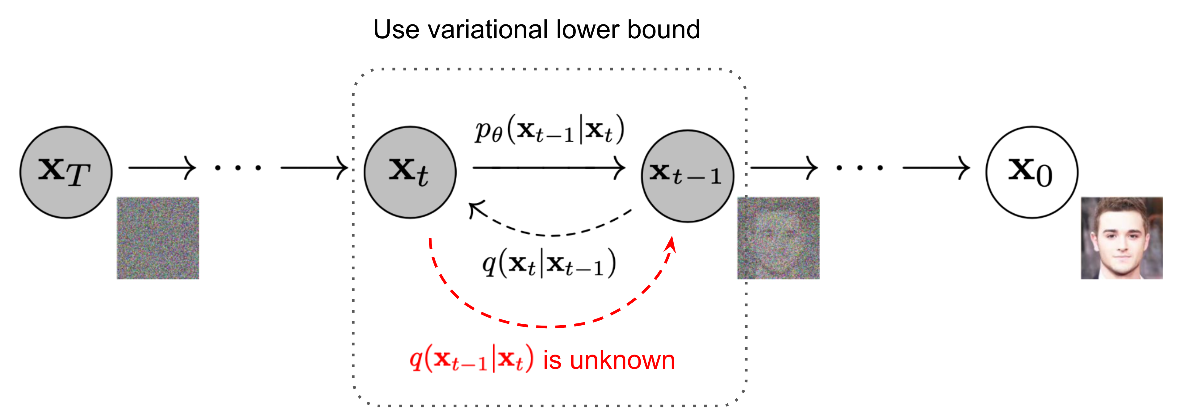
Diffusion models are inspired by non-equilibrium thermodynamics. They define a Markov chain of diffusion steps to slowly add random noise to data and then learn to reverse the diffusion process to construct desired data samples from the noise. Unlike VAE or flow models, diffusion models are learned with a fixed procedure and the latent variable has high dimensionality (same as the original data).

Diffusion models은 비평형 열역학(non-equilibrium thermodynamics)^[4]에서 영감을 받았다. 그들은 데이터에 랜덤 노이즈를 천천히 추가하는 Markov chain of diffusion steps를 정의한 후에 노이즈로부터 원하는 데이터 샘플(input $x$)를 구성하기 위해 diffusion process를 역순으로 학습한다. VAE와 Flow-based 모델들과 달리, Diffusion모델은 fixed procedure(고정된 순서)대로 학습되고 latent vairable(잠재 변수)는 고차원성(원본 데이터와 같은)을 가진다.

1. Non-equilibrium thermodynamics
   • 비평형 열역학(Non-equilibrium thermodynamics)은 열역학의 균형 상태(equilibrium state)^[5]와 달리, 시스템이 균형을 유지하지 않는 상태에서 열역학적인 성질을 연구하는 분야입니다. 균형 상태의 열역학과는 다르게 시간에 따라 변화하는 상태를 분석하기 때문에, 복잡한 시스템에서 유용하게 사용됩니다. 지역 평형 가정을 바탕으로 한 균형 상태에서의 열역학을 확장하는 방식으로, 비평형 열역학을 연구하는 것이 일반적입니다[4-1][4-2].
2. equilibrium state(평형 상태)
   • 화학, 역학 등의 분야에서 사용되는 ‘평형 상태’는 닫힌 계에서 변화가 없는 상태를 말합니다. 이 때, 반응물과 생성물의 농도가 같으며, 계 내에 자유에너지의 출입이 없습니다. 엔트로피는 일정하며, 정상 상태 반응에서는 특정 반응물의 생성과 소멸 속도가 일정합니다. 계는 닫힌계 혹은 열린계에서 전체가 아닌 일부 상태변수가 일정하며, 계 내에 자유에너지는 지속적으로 투입됩니다. 엔트로피는 증가합니다. [5-1][5-2] 한편, 물리학에서 사용되는 ‘정적 평형 상태’는 어떤 계의 모든 성분에 대한 힘과 돌림힘 각각의 합이 0이 되는 상태를 의미합니다. 이러한 계는 정역학에서 다루어지며, 예를 들어 책상 위의 문진을 생각해 볼 수 있습니다. [5-3]

Fig. 1. Overview of different types of generative models.

What are Diffusion Models?

Several diffusion-based generative models have been proposed with similar ideas underneath, including diffusion probabilistic models (DPM; Sohl-Dickstein et al., 2015), noise-conditioned score network (NCSN; Yang & Ermon, 2019), and denoising diffusion probabilistic models (DDPM; Ho et al. 2020).</p>

몇몇의 diffusion-based 생성 모델들은 diffusion probabilistic models (DPM; Sohl-Dickstein et al., 2015), noise-conditioned score network (NCSN; Yang & Ermon, 2019), 그리고 denoising diffusion probabilistic models (DDPM; Ho et al. 2020)들을 포함한 유사한 아이디어들을 바탕으로 제안되었다.

Forward diffusion process

Given a data point sampled from a real data distribution $\mathbf{x}0 \sim q(\mathbf{x})$, let us define a forward diffusion process in which we add small amount of Gaussian noise to the sample in $T$ steps, producing a sequence of noisy samples $\mathbf{x}_1, \dots, \mathbf{x}_T$. The step sizes are controlled by a variance schedule ${\beta_t \in (0, 1)}{t=1}^T$.

실제 data의 분포 $\mathbf{x}_0 \sim q(\mathbf{x})$로부터 sample된 data point가 주어졌을 때, 우리는 $T$ step들 마다 sample에 매우 작은 양의 Gaussian noise를 추가하여, noisy(노이즈가 추가된) sample $\mathbf{x}_1, \dots, \mathbf{x}_T$ sequence^[6]를 생산하는 forward diffusion process를 정의한다.

1. Sequence in deep learning?
   • 시퀀스(Sequence)란 일상생활에서 시간에 따라 변화하는 모든 것을 말합니다. 따라서 텍스트, 음성, 비디오 등의 순차 데이터(sequential data)에 대한 머신러닝(Machine Learning)을 수행하려면 일반적인 인공신경망(Artificial Neural Network)을 사용하여 전체 시퀀스를 입력으로 제공할 수 있습니다. 그러나 데이터의 입력 크기가 고정되어 있기 때문에 제한적인 한계가 있습니다[6-1]. 딥러닝 전문화 과정에서는 시퀀스 모델(sequence model)과 음성 인식, 음악 합성, 챗봇, 기계 번역, 자연어 처리(Natural Language Processing, NLP) 등의 흥미로운 응용 분야에 대해 다루며, Recurrent Neural Networks(RNNs)를 구축하고 학습할 수 있는 능력을 갖출 수 있습니다[6-2]. Sequence to Sequence Learning with Neural Networks는 Deep Neural Networks(DNNs) 모델이 어려운 학습 작업에서 우수한 성능을 보이지만, 시퀀스를 시퀀스로 매핑하는 데 사용할 수 없다는 문제점을 제시합니다. 이 논문에서는 일반적인 end-to-end 방법론을 제안하여 DNNs 모델이 시퀀스를 시퀀스로 매핑할 수 있도록 합니다[6-3]. \(q(\mathbf{x}_t \vert \mathbf{x}_{t-1}) = \mathcal{N}(\mathbf{x}_t; \sqrt{1 - \beta_t} \mathbf{x}_{t-1}, \beta_t\mathbf{I}) \quad q(\mathbf{x}_{1:T} \vert \mathbf{x}_0) = \prod^T_{t=1} q(\mathbf{x}_t \vert \mathbf{x}_{t-1})\)

The data sample $\mathbf{x}_0$ gradually loses its distinguishable features as the step $t$ becomes larger. Eventually when $T \to \infty$, $\mathbf{x}_T$ is equivalent to an isotropic Gaussian distribution.

$t$ 단계가 커짐에 따라 데이터 샘플 $\mathbf{x}_0$는 점차 구별 가능한 feature들을 잃는다. 결국 $T \to \infty$일 때, $\mathbf{x}_T$는 isotropic Gaussian distribution(등방성 가우시안 분포)^[7]와 같다.

1. isotropic Gaussian distribution(등방성 가우시안 분포)
   • 등방성 가우시안 분포란, 확률밀도 함수가 회전에 대해 불변^[8]하며, 분산-공분산 행렬이 항등행렬인 가우시안 분포를 의미합니다. [7-1][7-3] 정규분포란 연속 확률 분포 중에서 가장 널리 알려진 분포 중 하나이며, 다변량 가우시안 분포는 입력 변수가 D차원의 벡터인 경우에 사용됩니다. [7-2] 따라서, 등방성 가우시안 분포는 분산-공분산 행렬이 항등행렬인 가우시안 분포를 말하며, 이는 회전에 대해 불변합니다. 이러한 특징 때문에, 등방성 가우시안 분포는 확률 분포 중에서 가장 간단하면서도 많은 곳에서 유용하게 사용됩니다. [7-1][7-3]
2. 확률 밀도 함수가 회전에 대해 불변하다.
   • 확률밀도 함수가 회전에 대해 불변(invariant)하다는 것은, 3차원 공간에서 특정한 방향으로 회전하더라도 확률밀도 함수가 변하지 않는다는 의미입니다. 이는 3차원 공간에서 확률밀도 함수가 벡터가 아니라 스칼라인 경우에 해당합니다. 확률밀도 함수가 회전에 대해 불변하다는 것은 다음과 같이 정의됩니다. 만약 확률밀도 함수 p(x)가 회전 변환 T에 대해 불변하다면, 임의의 회전 변환 T에 대해 다음이 성립합니다.$∫p(Tx)dV = ∫p(x)dV$ 여기서 x는 3차원 공간에서 위치를 나타내는 벡터이고, dV는 부피 요소입니다.즉, 확률밀도 함수가 회전에 대해 불변하다는 것은, 어떤 방향으로 회전해도 확률밀도 함수의 모양이 변하지 않는다는 것을 의미합니다. 이는 회전에 대한 불변성이라고도 합니다. [8-1]</p>

Fig. 2. The Markov chain of forward (reverse) diffusion process of generating a sample by slowly adding (removing) noise. (Image source: Ho et al. 2020 with a few additional annotations)

A nice property of the above process is that we can sample $\mathbf{x}_t$ at any arbitrary time step $t$ in a closed form using reparameterization trick.

위 프로세스에서 좋은 변수는 reparameterization trick^[9]을 사용한 closed form의 임의의 time step $t$에서 $\mathbf{x}_t$을 samle할 수 있다.

1. Reparameterization trick
   • Reparameterization trick(재매개변수화 기법)은 Variational Autoencoder(VAE)에서 사용되는 기법으로, stochastic node를 deterministic한 부분과 stochastic한 부분으로 분해하여 backpropagation을 계산하기 쉽게 만드는 기법입니다. 즉, $x = g (ϕ, ϵ)$로 deterministic, stochastic의 함수로 나타내어 backpropagation을 수행합니다. 예를 들어, $x ∼ N ( μ ϕ, σ ϕ 2)$ 인 경우, $ϵ ∼ N (0, 1)$을 이용하여 $x = μ ϕ + σ ϕ 2 ∗ ϵ$으로 표현할 수 있습니다. 이를 통해 모델이 학습할 수 있는 deterministic한 부분과 확률적인 부분을 분리하고, 더욱 정확한 학습이 가능해집니다. 이 기법은 VAE뿐만 아니라, 다른 Autoencoder에서도 유용하게 사용될 수 있습니다. 자세한 내용은 [9-1], [9-2], [9-3]를 참고하시면 됩니다.

Let $\alpha_t = 1 - \beta_t$ and $\bar{\alpha}t = \prod{i=1}^t \alpha_i$:

\[\begin{aligned} \mathbf{x}_t &= \sqrt{\alpha_t}\mathbf{x}_{t-1} + \sqrt{1 - \alpha_t}\boldsymbol{\epsilon}_{t-1} & \text{ ;where } \boldsymbol{\epsilon}_{t-1}, \boldsymbol{\epsilon}_{t-2}, \dots \sim \mathcal{N}(\mathbf{0}, \mathbf{I}) \\ &= \sqrt{\alpha_t \alpha_{t-1}} \mathbf{x}_{t-2} + \sqrt{1 - \alpha_t \alpha_{t-1}} \bar{\boldsymbol{\epsilon}}_{t-2} & \text{ ;where } \bar{\boldsymbol{\epsilon}}_{t-2} \text{ merges two Gaussians (*).} \\ &= \dots \\ &= \sqrt{\bar{\alpha}_t}\mathbf{x}_0 + \sqrt{1 - \bar{\alpha}_t}\boldsymbol{\epsilon} \\ q(\mathbf{x}_t \vert \mathbf{x}_0) &= \mathcal{N}(\mathbf{x}_t; \sqrt{\bar{\alpha}_t} \mathbf{x}_0, (1 - \bar{\alpha}_t)\mathbf{I}) \end{aligned}\]

Reference

[1-1] “An example of a surrogate loss function could be $psi (h (x)) = max (1 - h (x), 0)$ (the so-called hinge loss in SVM), which is convex and easy to optimize using conventional methods. This function acts as a proxy for the actual loss we wanted to minimize in the first place. Obviously, it has its disadvantages, but in some cases a surrogate …” URL: https://stats.stackexchange.com/questions/263712/what-is-a-surrogate-loss-function

[2-1] “We introduce Glow, a reversible generative model which uses invertible 1x1 convolutions. It extends previous work on reversible generative models and simplifies the architecture. Our model can generate realistic high resolution images, supports efficient sampling, and discovers features that can be used to manipulate attributes of data.” URL: https://openai.com/blog/glow/

[2-2] “These can also be described as flow-based models, reversible generative models, or as performing nonlinear independent component estimation. … This transform is where Invertible 1x1 …” URL: https://medium.com/ai-ml-at-symantec/introduction-to-reversible-generative-models-4f47e566a73

[2-3] “Reversible Architectures are a family of neural network architectures that are based on the NICE [12,13] reversible transformation model which are the precursors of the mod-ern day generative flow based image generation architec-tures [29,36]. Based on the NICE invertible transforma-tions, Gomez et al. [22] propose a Reversible ResNet ar-“ URL: https://openaccess.thecvf.com/content/CVPR2022/papers/Mangalam_Reversible_Vision_Transformers_CVPR_2022_paper.pdf

[3-1] “Formally speaking, there are two conditions that must be satisfied in order for a function to have an inverse. 1) A function must be injective (one-to-one). This means that for all values x and y in the domain of f, f (x) = f (y) only when x = y. So, distinct inputs will produce distinct outputs. 2) A function must be surjective (onto).” URL: https://www.khanacademy.org/math/precalculus/x9e81a4f98389efdf:composite/x9e81a4f98389efdf:invertible/v/determining-if-a-function-is-invertible

[3-2] “Learn how to find the formula of the inverse function of a given function. For example, find the inverse of f (x)=3x+2. Inverse functions, in the most general sense, are functions that reverse each other. For example, if f f takes a a to b b, then the inverse, f^ {-1} f −1, must take b b to a a.” URL: https://www.khanacademy.org/math/algebra-home/alg-functions/alg-finding-inverse-functions/a/finding-inverse-functions

[4-1] “2.1 Quasi-radiationless non-equilibrium thermodynamics of matter in laboratory conditions 2.2 Local equilibrium thermodynamics 2.2.1 Local equilibrium thermodynamics with materials with memory 2.3 Extended irreversible thermodynamics 3 Basic concepts 4 Stationary states, fluctuations, and stability 5 Local thermodynamic equilibrium” URL: https://en.wikipedia.org/wiki/Non-equilibrium_thermodynamics

[4-2] “The extension of equilibrium thermodynamics to nonequilibrium systems based on the local equilibrium assumption is a well-accepted practice in nonequilibrium thermodynamics. 3.3 STATIONARY STATES Intensive properties that specify the state of a substance are time independent in equilibrium systems and in nonequilibrium stationary states.” URL: https://courses.physics.ucsd.edu/2020/Fall/physics210b/Non-Eqbrm%20Thermo_Demirel%20and%20Gerbaud.pdf

[5-1] “평형 (Equilibrium)과 정상 상태 (Steady State) 평형 이란, 닫힌계에서 변화가 없는 것을 말하며 반응물과 생성물의 농도가 같다. 계 (System) 내에 자유에너지의 출입이 없다. 엔트로피 일정하다. 정상 상태 반응에서 특정 반응물의 생성과 소멸 속도가 일정하다. 닫힌계 혹은 열린계에서 전체가 아닌 일부 상태변수가 일정하다. 계 내에 자유에너지는 지속적으로 투입된다. 엔트로피는 증가한다. CASLAB조인진 화학반응과 평형상태 과정 출처 : Pinterest 마지막으로 일상생활 및 인문학적으로 평형과 정상상태를 생각해 보면 이렇습니다.” URL: https://blog.naver.com/PostView.nhn?blogId=welcomelady&logNo=222224467182

[5-2] “화학 평형 (化學 平衡, 영어: chemical equilibrium )은 화학 반응 에 있어서 정반응 속도와 역반응 속도가 같아져 겉보기에 화학 반응이 일어나지 않는 것처럼 보이는 상태이다. 상당수의 화학 반응에서 반응물 이 생성물 로 완전히 변하지 않고, 결과적으로 화학 평형 상태를 유지한다. 화학 평형에 도달하게 되면 온도, 압력 등의 실험 환경이 변하지 않는 이상, 반응물과 생성물의 양이 변하지 않는다. [1] 화학 평형 상태는 동적 평형 상태 로, 거시적으로는 반응물과 생성물의 양이 변화하지 않으나 실제로 반응은 계속 일어나고 있는 상태이다.” URL: https://ko.wikipedia.org/wiki/%ED%99%94%ED%95%99_%ED%8F%89%ED%98%95

[5-3] “정적 평형 상태 (Equilibrium)는 입자의 알짜힘 이 0인 상태 [1] :39, 즉 어떤 계의 모든 성분에 대한 힘 과 돌림힘 각각의 합이 0이 되는 상태를 의미한다. 이러한 계는 정역학 에서 다루어진다. 예로써, 책상 위의 문진을 생각해 보자. 관성 기준틀을 방의 운동과 일치하도록 선택한다면, 책상과 문진의 계는 바닥에 대해 정적 평형 상태에 있다고 볼 수 있다. 관성 기준틀을 방의 운동에 일치하도록 선택했으므로, 지구의 움직임에 의한 작은 가속도 ( 코리올리 힘, 구심 가속도 를 참조)는 무시할 수 있다. 같이 보기 [ 편집] 가상일의 원리 동적 평형 상태 부정정 준안정 학문 물리학 역학 (물리학) 고전역학” URL: https://ko.wikipedia.org/wiki/%EC%A0%95%EC%A0%81%ED%8F%89%ED%98%95%EC%83%81%ED%83%9C

[6-1] “Sequence Learning Everything in life depends on time and therefore, represents a sequence. To perform machine learning with sequential data (text, speech, video, etc.) we could use a regular neural network and feed it the entire sequence, but the input size of our data would be fixed, which is quite limiting.” URL: https://developer.nvidia.com/blog/deep-learning-nutshell-sequence-learning/

[6-2] “In the fifth course of the Deep Learning Specialization, you will become familiar with sequence models and their exciting applications such as speech recognition, music synthesis, chatbots, machine translation, natural language processing (NLP), and more. By the end, you will be able to build and train Recurrent Neural Networks (RNNs) and …” URL: https://www.coursera.org/learn/nlp-sequence-models

[6-3] “Sequence to Sequence Learning with Neural Networks. Deep Neural Networks (DNNs) are powerful models that have achieved excellent performance on difficult learning tasks. Although DNNs work well whenever large labeled training sets are available, they cannot be used to map sequences to sequences. In this paper, we present a general end-to-end …” URL: https://arxiv.org/abs/1409.3215

[7-1] “Isotropy can refer to invariance under rotation, or that the covariance matrix is the identity. (Those two are generally not the same). A reference for the first definition is Stochastic and Integral Geometry by Schneider Weil, a reference for the second is High-Dimensional Probability by Roman Vershynin. - Idontgetit Feb 8 at 9:07” URL: https://math.stackexchange.com/questions/1991961/gaussian-distribution-is-isotropic

[7-2] “The Gaussian Distribution [I] 가우시안 분포는 보통 정규분포(standard distribution)로 알려져있다. 왜냐하면 연속 확률 분포 중 가장 널리 알려진 분포이기 때문이다. 단일 변수 ( x ) 에 대해 가우시안 분포는 다음과 같이 기술된다. 여기서 ( mu ) 는 평균, ( sigma^2 ) 은 분산이다. 입력 변수가 ( D ) 차원의 벡터인 경우를 다변량 가우시안 분포라 하며 다음과 같은 식으로 기술한다.” URL: http://norman3.github.io/prml/docs/chapter02/3_1.html

[7-3] “그러면 먼저 가우시안 분포 f(x) f ( x) 가 e−x2 e − x 2 형태의 꼴을 따르는 ① 식을 살펴보겠습니다. 이 식의 전개를 살펴보기 위하여 직교좌표계 와 극좌표계 의 관계를 이용해야하기 때문에 다음과 같은 가정을 사용합니다. ⓐ 원점으로 같은 거리에 있는 점은 확률 값은 모두 같으므로 확률 밀도 함수는 회전 각도에 독립적 입니다. ⓑ 사각형의 크기가 같을 때, 원점으로부터 사각형까지의 거리가 가까울수록 그 사각형의 확률밀도는 높습니다. ⓒ 사각형까지의 거리가 같을 떄에는 사각형의 넓이가 넓을 수록 확률밀도가 높습니다.” URL: https://gaussian37.github.io/math-pb-about_gaussian/

[8-1] “확률론 에서 확률 밀도 함수 (確率密度函數, 영어: probability density function 약자 pdf)는 확률 변수 의 분포 를 나타내는 함수 로, 확률 밀도 함수 와 구간 에 대해서 확률 변수 가 구간에 포함될 확률 는 가 된다. 확률 밀도 함수 는 다음의 두 조건을 만족해야 한다. 모든 실수 값 에 대해 확률 밀도 함수와 누적 분포 함수 에는 다음과 같은 수식이 성립한다. 전거 통제: 국립도서관 이 글은 수학에 관한 토막글 입니다. 여러분의 지식으로 알차게 문서를 완성해 갑시다.” URL: https://ko.wikipedia.org/wiki/%ED%99%95%EB%A5%A0%EB%B0%80%EB%8F%84%ED%95%A8%EC%88%98

[9-1] “Reparameterization trick VAE에서 보던 trick인데, 굉장히 단순하며 잘 작동한다. stochastic node를 stochastic한 부분과 deterministic한 부분으로 분해시켜서 deterministic한 부분으로 backpropagation을 흐르게하자는게 핵심! 즉, x = g ( ϕ, ϵ) 로 deterministic, stochastic의 함수로 본다. 예를 들어보면 x ∼ N ( μ ϕ, σ ϕ 2) 인 녀석은 ϵ ∼ N ( 0, 1) 을 이용하면 x = μ ϕ + σ ϕ 2 ∗ ϵ 으로 나타낼 수 있다.” URL: https://hulk89.github.io/machine%20learning/2017/11/20/reparametrization-trick/

[9-2] “The reparameterization trick is a powerful engineering trick. We have seen how it works and why it is useful for the VAE. We also justified its use mathematically and developed a deeper understanding on top of our intuition. Autoencoders, more generally, is an important topic in machine learning.” URL: https://www.baeldung.com/cs/vae-reparameterization

[9-3] “Reparameterization trick is a way to rewrite the expectation so that the distribution with respect to which we take the gradient is independent of parameter $theta$. To achieve this, we need to make the stochastic element in $q$ independent of $theta$.” URL: https://stats.stackexchange.com/questions/199605/how-does-the-reparameterization-trick-for-vaes-work-and-why-is-it-important